1.2.4 - Data Storage - Encoding Sound
The final stop on our encoding journey is sound. In this section we learn how sound waves are translated into a digital, binary form and conversely, how a computer transforms digital data back in to analogue sound.
If you have studied image encoding, you will have noticed that not everything in computing and encoding is perfect. As with images, sound encoding involves a number of trade offs and compromises between the quality of the final sound and the amount of data we produce. How far you can take that compromise depends on the intended use of the sound. For example, we do not need CD quality audio to play the slightly irritating plinky-plonk hold music you get when you phoning a call centre.
In this section (click to jump):
What is sound?
Sound is a vibration. Depending on the frequency of those vibrations, we can hear the sound as different tones. The vibrations that create sounds can be represented as waves, like the one shown below:
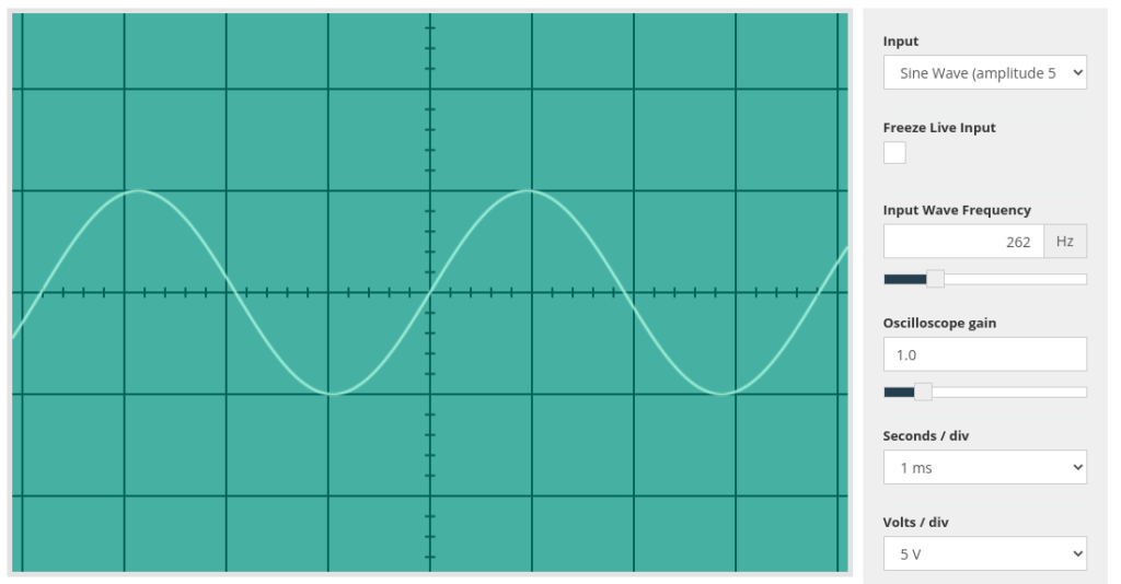
If you remember right back to how the speed of a CPU is measured, we use Hertz to describe how often something happens in one second. Therefore the sound above, at 262 Hz means a vibration happening 262 times per second. The human ear is capable of hearing sounds that range from 20Hz all the way up to 20Khz (20,000 Hz) which is effectively the lowest rumble you can imagine to the highest, ear piercing high pitched squeal.
When a speaker creates a sound, it moves backwards and forwards effectively punching the air. It creates areas of high pressure as it moves out and low pressure as it moves back again. This forwards and backwards movement creates waves in the air molecules that we hear as sound. If you were to look at the graph of a sound wave, the high pressure is represented as peaks in the wave, the low pressure is where the wave dips.
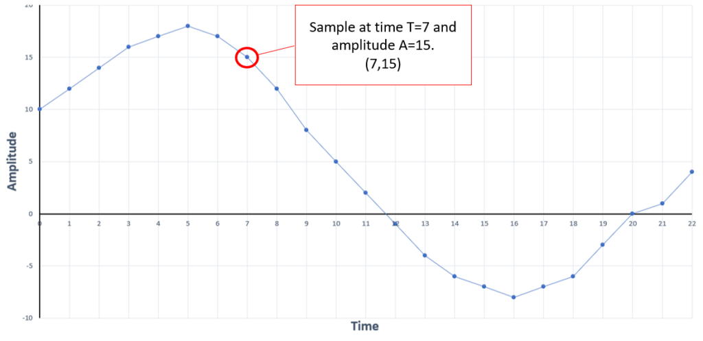
The key to understanding how a computer can encode, decode and store sound as binary data lies in the fact that we can represent all sound on a graph, we can plot the "wave" that represents any sound. As you will know from your maths lessons, you can plot a graph using X and Y co-ordinate pairs. The opposite is also true, using graph paper you can draw a line and then convert that into co-ordinate pairs by selecting regular points along the line and working out where they are on the X and Y axis.
Samples
The goal of encoding any form of data is to translate it into binary form. Therefore we need a method of converting an analogue sound wave into numbers - ones and zeroes. Fortunately at GCSE level we largely ignore the process of actually capturing the sound as carried out by a microphone. Microphones capture the vibrations of a sound and create an electrical signal from this. This signal is then fed into a magic box called an "analogue to digital converter" which turns the signal into digital data.
We need to understand how that conversion takes place.
To store a sound wave as data we need to do two things:
- Decide how often to measure the amplitude (height) of the sound wave
- Decide how many binary bits to use to store both amplitude and time data
A single point on the sound wave line is called a sample. The number of times we record a sample per second is called the "sampling rate." Here lies our first trade off in sound encoding. In order to record the highest quality sound file, you need to take as many samples per second as possible. However, the more samples you take, the more data you generate and the larger a sound file will become.
In real world sound recording, it is necessary to take many thousands of samples per second even for poor quality audio. Below is a selection of common audio formats and their sampling rates:
| Sampling Rate (number of samples per second) | Audio application and comments |
| 8000hz | Telephone or basic voice recordings. Poor quality, can be some distortion. |
| 44,100hz | CD quality audio |
| 96,000hz | Blu-Ray or HD-DVD audio tracks, DVD-audio. Extremely high quality sound |
As can be seen above, even for the most basic quality of sound, 8000 samples per second are required to store and reproduce speech. For CD quality audio over 44 thousand samples per second are used - just take a moment to think about the sheer quantity of binary data this is creating just for a single second of sound.
The sampling rate, however, is just one side of the story - the X axis, if you like. The Y axis records the amplitude of the wave. The number of possible values for the amplitude of the wave is dictated by the number of binary bits that are allocated to this purpose. This, as with image encoding, is called "bit depth."
Just as we saw with image encoding where bit depth affects how many colours we can display, audio bit depth affects how accurately we can record the amplitude of the sound wave and therefore how close to the original that sound will be.
CD audio allocates 16 bits per sample for the bit depth of each sample. It is estimated that approximately 21 bits per sample would be needed to accurately record the entire range of human hearing from 20hz to 20Khz, so arguably some information is lost in a CD quality recording although you would need the hearing of Batman in order to actually notice. It is far more likely the quality of your audio equipment will negatively affect the sound before you can hear any defects in a CD recording.
Sound quality
Using the information above, we can summarise that audio encoding is nothing more than a collection of samples, X and Y co-ordinates effectively. The quality of those samples and the resulting sound is down to these two factors:
- Sampling rate - how many times per second we record data
- Bit depth - how accurately the amplitude of the wave can be recorded in each sample
From this, we can do some maths to work out just how much data is created when encoding a sound.
Taking CD quality as the benchmark, we know that there are:
- 44,100 samples per second
- 16 bits of data to record amplitude per sample
Therefore, in 1 second of audio, there are 44,100 * 16 = 705,600 BITS of data.
Using our conversions from Unit 1.3, we can work out that 705,600 bits equates to:
- 705,600 / 8 = 88,200 Bytes of data
- 88,200 / 1024 = 86 Kb of data
So, one single second of audio, at CD quality, takes up 86Kb of storage. For one minute of audio that's:
- 88,200 bytes * 60 seconds = 5,292,200 bytes
- 5,292,200 bytes / 1024 = 5,167.97 KB
- 5,167 KB is roughly 5MB
Whilst today we think nothing of sending 5mb of data to a friend in the form of a photograph or the latest meme, this is still a fairly large chunk of binary data. As such there are many clever methods that have been created to compress or reduce the amount of data that is created by encoding audio.
For the GCSE we simply need to be aware that there are two obvious ways in which the amount of data could be reduced:
- Change or reduce the number of samples per second - sampling rate
- Reduce the amount of bits allocated per sample - bit depth
You knew, didn't you, that there would be a trade off in doing these two things? The relationship is quite straight forward:
- If you reduce the sampling rate, fewer samples are created. A lower number of samples = less data.
- However, fewer samples mean it is harder to reproduce the original sound, therefore quality is lost.
- If you reduce the bit depth, less data per sample is created
- However, lower bit depth means less accurate representation of the sound and, you guessed it, quality is lost.
There is a clear relationship between the amount of data we create through encoding (file size) and the quality of the sound. Remember, no digital sound encoding is a 100% perfect recreation of the original sound that was created. However, we can get extremely close and when we talk about the quality of a sound what we really mean is "how close the recording is to the original sound?"
Finally, you should be aware of when and why we may reduce file size and quality. Some of the most common are outlined below:
- To reduce the file size - literally to take up less storage space with each sound file
- To reduce bandwidth used - sending data across the internet takes time and costs money. By reducing the file size, less data is transmitted.
- To compromise between speed and reliability of transmission and quality (streaming) - when streaming it is more important to maintain a constant stream of data than it is to have the highest possible quality sound. Algorithms will automatically increase or decrease quality based on the connection between host and client.
- When high quality is unnecessary - for example when listening to hold music on a telephone call. Telephones do not have the capability to reproduce high quality audio, so there is no point using a high quality file for this purpose.

